Don't miss out
Subscribe to QuickBooks for only
$1/month for 3 months
Don't miss out
Claim now
April Sale
Buy now and pay only $1/month
for your first 3 months
March into savings Don't miss out!
$1 /monthfor 3 months
Track your expenses as you go and save 11 hours of admin per week
QuickBooks Online $1 /monthfor 3 months
Start fresh this new year
with QuickBooks Online
$1 /monthfor 3 months
Sale ends soon. Don't miss out, sign up today
$1 /monthfor 3 months
Start fresh this new year
with QuickBooks Online
$1 /monthfor 3 months
$1/month
for 3 months
$1/month
for 12 months
When purchased in bundles of 10
50 %off for 3 months
50 %off for 12 months
  • Invoices
  • Expenses
  • Reports
Image Alt Text
Accounting and bookkeeping

10 Simple Microsoft Excel Tricks, Shortcuts and Hacks That Can Make You an Expert

Microsoft Excel is an integral part of most businesses. Some people relish the capabilities of Excel, finding it a useful tool that allows them to easily manage, report on and illustrate tables of data.

Others, however, find it tedious and downright obtuse, unable to make heads or tails of what exactly Excel can do from them, aside from keeping things in neat columns and rows.

Below is a list of 10 easy tricks, shortcuts and hacks that will put you on the path to being an Excel super user.

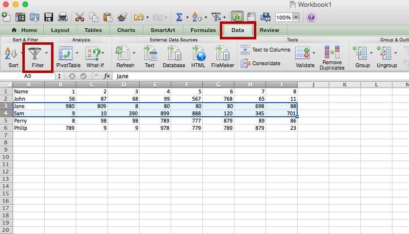
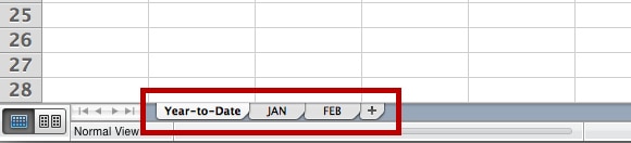
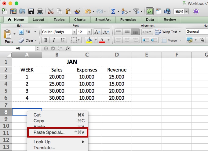
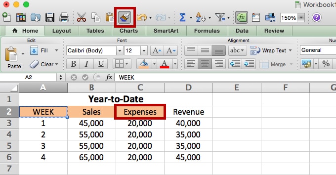
(Note: There are a many versions of Excel, including versions for desktop (Windows, Mac OS X) and mobile (iOS and Android) operating systems. The visuals are screenshots from a Mac version of Excel. These tips were confirmed to work on a Mac and Windows desktop, but may apply to other versions as well. This piece also discusses keyboard shortcuts for use in a Windows OS. For Mac, replace the “Control” key with the “Command” key.)


1. Select All Cells in a Spreadsheet at Once

Do you need to reformat your font or make some other sweeping change to your Excel workbook? An easy way to select all the cells in the document is to click on the square in the upper left-hand corner where the top of the rows and columns meet.

Image 1 – Click on the circled square to select all the cells in the workbook.

Clicking on this box will highlight all of the cells in the document, even empty cells.

If you prefer keyboard shortcuts, you can also select all cells by pressing the “Control” and “A” buttons at the same time.


2. Copy a Worksheet From 1 Workbook to Another

This is helpful if you’re looking to merge data across two workbooks together and don’t want to reformat all of your data in either workbook.

1. Start by opening your “source” workbook (the one with the data you want to copy).

2. Next, open your “target” workbook (you want to copy to). This can be a new workbook or an existing workbook.

3. In your source workbook, look towards the bottom left-hand corner and find the name of the sheet you want to copy. Unless the name of the worksheet is changed, it should have a name like “Sheet1” or something else.

4. Right-click on the sheet you want to copy (if on a Mac with a single-button mouse, you may need to hold down the Control key while clicking).

5. Select “Move or Copy …” from the menu.

Image 2 – Right-click (PC) or CTRL-Click (Mac) to reveal the menu. Select Move or Copy.

6. From the list, select where you want to move or copy the sheet to. You’ll need to click on the dropdown at the top to see other open workbooks.

Image 3 – Click on the circled arrow to see all of the available workbooks you can move or copy sheets to. This field defaults the workbook you’re currently in.

7. Choose the workbook to copy it to and where in the order of the existing worksheets you want it to be.

Alternatively, you can simply move the worksheet from one workbook to another by dragging it with your mouse, but it might be safer to copy it, at least until your comfort level with Excel increases.

3. Add Multiple Rows and/or Columns at Once

You might find you need to add multiple rows and columns at one time. For example, let’s say you want to add multiple rows in the middle of a set of data.

1. Select two rows, starting with the row directly below where you want the new rows to appear. (Note: You can choose as many rows as needed.)

2. Right-click (PC) or CTRL-click (Mac), and select “Insert” from the dropdown menu.


Image 4 – Highlight the rows, then right-click (or CTRL-click on Mac) to get the menu. Select Insert to add rows.

3. Your new rows will appear above the first row you selected.

Image 5 – The inserted rows will appear above the first row you selected.

Because you have highlighted rows, Excel understands that you want to insert rows and will insert the number highlighted. In this example, two rows have been highlighted, so two blank rows will appear once “Insert” is selected.


4. Filtering Data

By clicking on the “Data” tab at the top of the page and then clicking “Filter,” you will give each column it’s own clickable dropdown menu on each cell in the first row. Click one, and you can sort data in a variety of ways.


Image 6 – View of the Data menu and available options, including Sort and Filter.

From the list that appears, you can choose certain values or names. Simply unclick “Select All,” and then click on the names you want. Once you hit “OK,” the dropdown menu will disappear and show you just the names you had selected.

Image 7 – All of the available values in the cells will be selected when this menu is first opened. To start with a “clean slate,” simply uncheck “(Select All)” at the top of the list.


Image 8 – Select the values you want to see in this filtered view.

Image 9 – The information you excluded from this view has not been deleted, only temporarily hidden.

The list has now been truncated to include the values you chose. But as you can see by the circled row numbers, the other data has not been deleted; it is simply “hidden” in this view.

You can easily undo any sorting by clicking on the Filter button at the top and choosing “(Select All)” again.


5. Copying Figures From 1 Worksheet to Another in the Same Workbook

You can use a figure from one cell on one worksheet in another cell on another worksheet without having to copy and paste them. This is especially handy for calculations where a number might change month to month, but you have one worksheet that figures everything on a year-to-date basis.

1. The example below shows the first tab of the workbook that displays Year-To-Date sales, expenses and revenues totals.

2. The second tab is labeled JAN, and the third tab is labeled FEB.


3. To determine the sum, you need to enter the formula as circled below in the desired cell =SUM(JAN!B3+FEB!B3). The formula is “WorksheetName!WorksheetCell” without quotations.


Image 11 – You can enter the formula into the formula bar at the top of the screen (as circled) or directly into the cell.

Grow Your Business with QuickBooks

6. Copying a Formula Across Rows or Down Columns

You can copy any formula across a range of cells by simply using your mouse. Using the previous formula as an example, it only needed to be inputed once, in the B2 cell. Once it’s entered, click on the cell, and then click on the little box that appears in the lower right-hand corner. Drag it across the desired range of cells, and you will populate the range using the same formula.


Image 12 – This little box in the corner will not appear until you have entered the information in the cell and then tabbed away from it or clicked outside of it.


This copies the formula across the cells, but changes the values relative to the new cell’s position. For example, in the B3 cell, the formula will read “=SUM(JAN!B3+FEB!B3)” without quotes. In the C3 cell, the formula will read “=SUM(JAN!C3+FEB!C3)” and so on.

The same thing can be done if you drag the box downward instead of across; this copies the formula into the column. So the B3 column formula will read “=SUM(JAN!B3+FEB!B3)”, while the B4 formula will read “=SUM(JAN!B4+FEB!B4)”.


7. Transpose Columns and Rows

If you need to move pre-existing data from columns to rows—or vice versa—do not despair.

1. Select the data you want to transpose, and copy it (CTRL-C).

2. Click on the cell where you want to place the data, and then right-click to get the dropdown menu. From that menu, select “Paste Special…”.


Image 14 – Paste Special offers many different options than just transpose.

3. From the Paste Special menu, click “Transpose” in the lower right-hand corner, and then click OK.

4. The data is now flipped, with rows as columns and columns as rows.

8. Continuing a Series Down a Column or Across a Row

If you are inputting a numbered list, but don’t want to number every row, there’s a quick way to do it in Excel.

1. Start your series of numbers.


2. Next, click on the first cell in the list, and drag down on the small box in the lower right-hand corner (similar to #6.) The cells will auto-populate with what Excel believes you are trying to do. (It can be intuitive and figure out that it is a numbered list or a set of dates, etc.)

In the case below, you can see that it simply copied a 1 into each cell in the column, but that’s not what we want.


3. Click on the small box that appears, and select “Fill Series.”

4. This will adjust the values in the cells so that they become a numbered series. As shown below, this adjustment will be made for how many cells you have highlighted. So if you want it numbered from 1 to 100, just highlight the amount of cells you need.


9. Highlight a List of Numbers to See Basic Information

This is a favorite of many Excel super users, because it’s simple and so helpful, especially when dealing with figures and finances.

If you highlight a group of figures, Excel will display a few “facts” about them in the lower right-hand corner: namely, the number of cells that are highlighted, the total number of the cells and the average of the cells’ values.


This is really handy if you’re looking for quick total or average without having to enter a formula.


10. Other Essential Shortcut Keys and Tips

Here are some other shortcuts that you may not be aware of. Some of these are universal across all Microsoft Office products (e.g. Word, PowerPoint, etc.), but are still very helpful when using Excel.

  • Undo button: This little backwards arrow undoes the last action you took in the worksheet. It’s the graphic equivalent to using the CTRL-Z keyboard shortcut.


  • CTRL-SHIFT-Up or Down Arrow: Selects all of the cells directly above (up arrow) or below (down arrow) of the selected cell. (NOTE: This only selects cells above and below that have data).
  • SHIFT-F11: Creates a new worksheet in your current workbook called “Macro1.” (Note: In Mac OS, you may need to add the “Fn” key for this shortcut to work).
  • CTRL-Home: Navigates to cell A1.
  • CTRL-End: Navigates to the last cell that contains data.
  • Format Painter (the little paintbrush): Select the cell whose format you want to copy. Then click on Format Painter in the upper toolbar (or click on the paintbrush in the pop-up format menu that appears) and click on the cell you want to format. In the below example, we clicked on the “Expenses” cell, clicked on Format Painter and then clicked on “Revenue.”


As you’re starting a new business, it’s understandable to want to use spreadsheets to manage your finances. But as sales pick up and your numbers become increasingly complicated, it’s best to graduate to an easy-to-use accounting software. Sure, these tips will allow you to get a better handle of your Excel spreadsheets.

Our additional Excel tips and tricks for accounting will help you further refine the way you use Excel for your small business accounting, but the time saved and errors avoided by using financial software are well-worth the transition. Sign up for a 30-day free trial and see how QuickBooks Online can help you manage your small business accounting.


Related Articles