Ten Microsoft Excel tips and tricks to manage spreadsheets like a pro

Microsoft Excel is an integral business tool. Some people relish the capabilities of Excel, finding it to be a useful tool that allows them to easily manage, report on and illustrate tables of data. Others, however, find it tedious and are unable to discern what Excel can do for them aside from keeping things in neat columns and rows. Whether you’re analysing huge amounts of data or trouncing timesheet templates, Microsoft Excel management can provide the technological advantage you need to get the job done.

Are you the person who finds it confusing? That’s OK. We have some Excel tips that can make your life with this database multi-tool much easier and more productive. You might even have fun learning some Excel functions along the way. We’ll save you the Google search—read on to discover a list of 10 genius Excel tips and tricks.

Ten Excel tips and tricks

There are many versions of Excel, including versions for desktop (Windows, Mac OS X) and mobile (iOS and Android) operating systems. The visuals here are screenshots from the Mac version of Excel. These Excel tips have been confirmed to work on a Mac and Windows desktop but may apply to mobile versions as well. This piece also discusses keyboard shortcuts for use in Windows OS. For Mac, replace the Ctrl key with the Command key.

Whether you’re a beginner or looking for ways to create your perfect budget template, these tips can get you on top of your Excel game.

Excel trick no. 1: select all cells in a spreadsheet

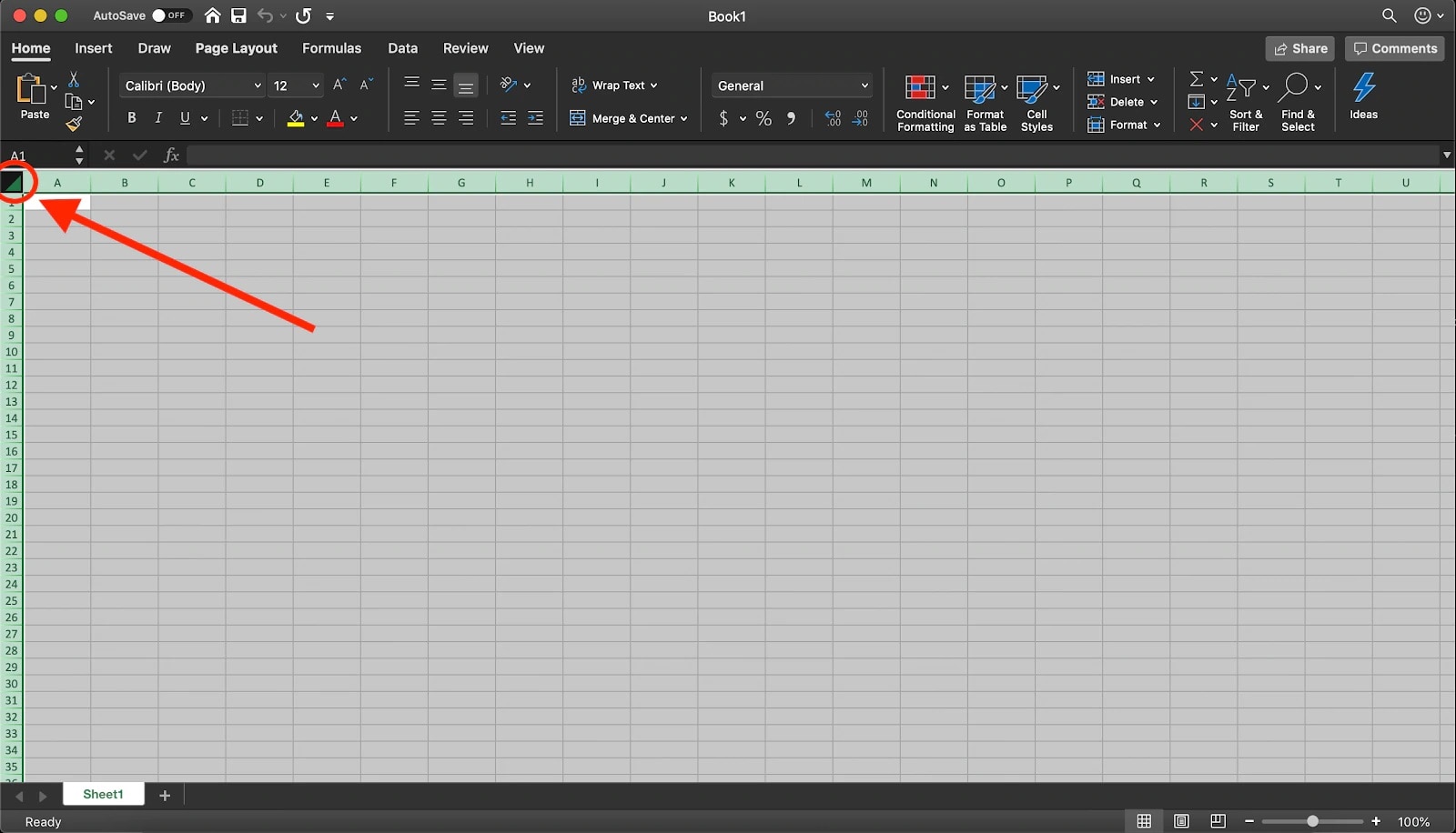
Do you need to reformat your font or make some other sweeping change to your Excel workbook? Click on the square in the upper left-hand corner to select all the cells in the workbook. You’ll find it where the top of the rows and columns meet. Clicking on this box will highlight all of the cells in the document, even empty cells.

If you prefer keyboard shortcuts, you can also select all cells if you press the Ctrl and A keys (Ctrl + A) at the same time. This is also a great way to format cells at once. Do you have a formula wrong or want to change a whole heap of cell rules? You can save a lot of time by making all these changes at once using the “Select All” function.

Pro Excel tip: use conditional formatting. Conditional formatting in Excel allows you to highlight cells of a certain colour, depending on the specified cell value. This is a great option for those who don’t necessarily need the structure of a VLOOKUP but want an organised look into their data sets.

Excel trick no. 2: copy a worksheet from one workbook to another

Have you ever been in an Excel file and suddenly realised you need to duplicate one or more large data sets? If you have a lot of formatting, manually entering this data is a nightmare.

This is where copying a worksheet from one workbook (a collection of multiple sheets) to another comes in.

1. Go to your “source” workbook (the one with the data you want to copy).

2. Open your “target” workbook (the one you want to copy to). This can be a new workbook or an existing workbook.

3. In your source workbook, look towards the bottom left-hand corner and find the name of the sheet you want to copy. Unless you’ve changed the name of the worksheet, it should have a name like “Sheet1”.

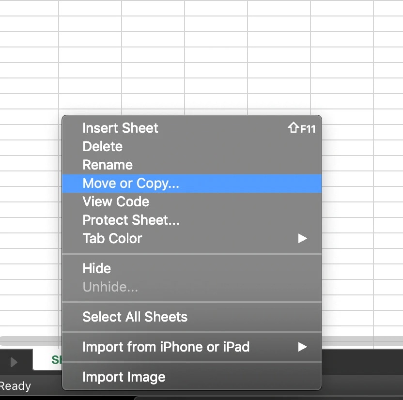
4. Right-click on the sheet you want to copy (if you’re on a Mac with a single-button mouse, you may need to hold down the Command key while clicking).

5. Select “Move or Copy…” from the menu.

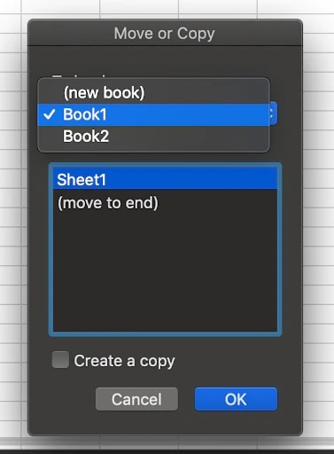
6. From the list, select where you want to move or copy the sheet to. You’ll need to go to the dropdown menu at the top to see other open workbooks.

7. Choose the workbook to copy it to and select where in the order of the existing worksheets you want it to be.

Alternatively, you can move the worksheet from one workbook to another by dragging it with your mouse. However, it might be safer to copy it, at least until your comfort level with Excel increases.

If you ever have extensive data validation to do and want to avoid botching a formula, try the copying method. It can be a quick and easy way to make a backup workbook.

Excel trick no. 3: add multiple rows or columns at once

You might find you need to add multiple rows and columns at one time. For example, let’s say you want to add two rows in the middle of a set of data. You’ll need to:

1. Select two rows, starting with the row directly below where you want the new rows to appear. (You can choose as many rows as needed. We’re just using two for this example.)
2. Right-click (PC) or Command-click (Mac) and select “Insert” from the dropdown menu.
3. Your new rows will appear above the first row you selected.

Because you’ve highlighted rows, Excel understands that you want to insert rows and will insert the number highlighted. In this example, we’ve highlighted two rows, so two blank rows will appear when you select “Insert”. If you highlight columns, this trick will work the same way.

Excel trick no. 4: filter data

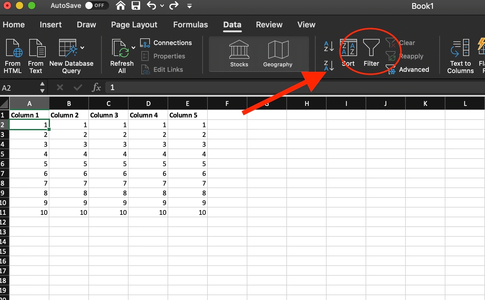
Select the “Data” tab at the top of the page, then select “Filter” to give each column its own clickable dropdown menu. The menu will appear on each cell in the first row. Select one, and you can sort data in a variety of ways.

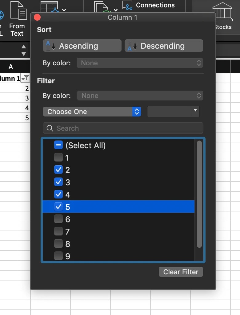
From the list that appears, you can choose certain values or names. Simply un-click “Select All”, then click on the names you want. Once you click “OK”, the dropdown menu will disappear and show you just the names you had selected.

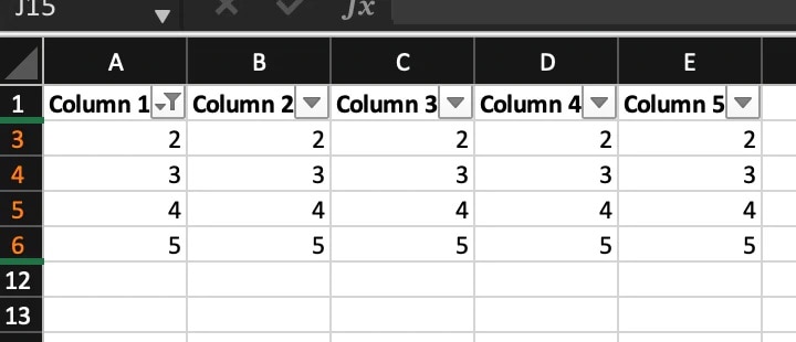
The list has now been truncated to include the values you chose. But as you can see by the circled row numbers, the other data hasn’t been deleted. It is simply “hidden” in this view.

You can easily undo any sorting by clicking on the “Filter” button at the top and choosing “Select All” again.

Excel trick no. 5: copy figures from one worksheet to another in the same workbook

You can use a figure from one cell on one worksheet in another cell on another worksheet without having to copy and paste it. This is especially handy for calculations where a number might change from month to month, but you have one worksheet that figures everything on a year-to-date basis.

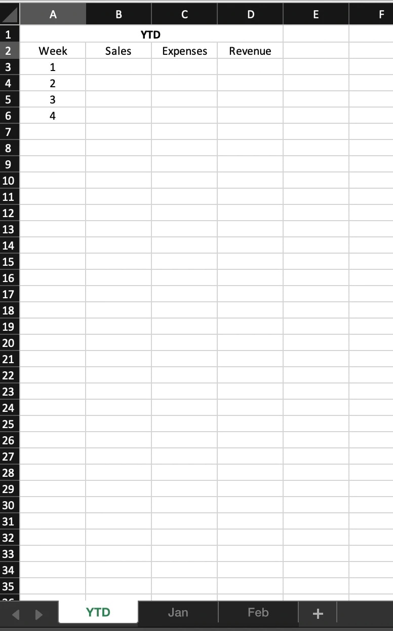
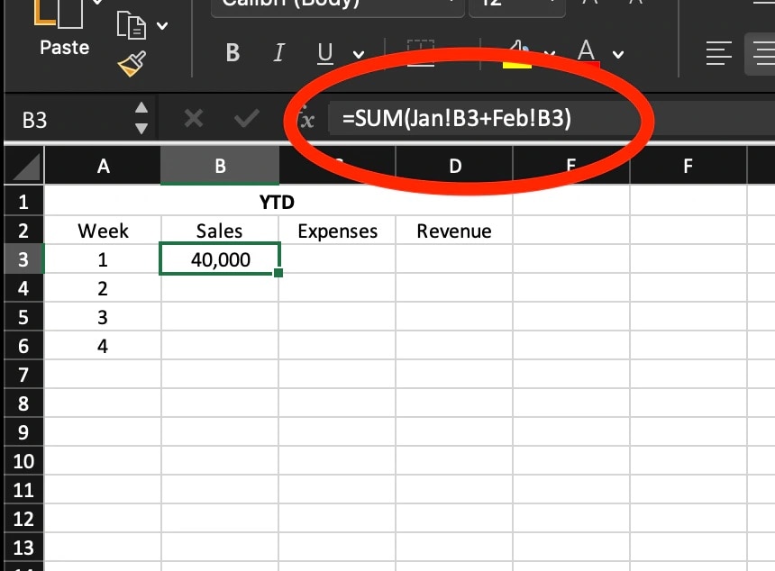
The example below shows the first tab of the workbook, which displays year-to-date sales, expenses and revenue totals.

The second tab is labeled JAN, and the third tab is labeled FEB. To determine the sum, you need to enter the following in the desired cell: =SUM(JAN!B3+FEB!B3). The formula is “WorksheetName!WorksheetCell” without quotes.

Excel trick no. 6: copy a formula across rows or down columns

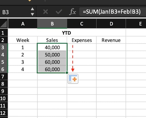
You can copy any formula across a range of cells using your mouse. With the previous formula as an example, it only needs to be input once, in the B2 cell. Once it’s entered, select the cell, then click on the little box that appears in the lower right-hand corner. Drag it across the desired range of cells, and you will populate the range using the same formula.

This copies the formula across the cells but changes the values relative to the new cell’s position. For example, in the B3 cell, the formula will read “=SUM(JAN!B3+FEB!B3)” without quotes. In the C3 cell, the formula will read “=SUM(JAN!C3+FEB!C3)” and so on.

You can do the same thing if you drag the box downwards instead of across. This copies the formula into the column. So the B3 column formula will read “=SUM(JAN!B3+FEB!B3)” and the B4 formula will read “=SUM(JAN!B4+FEB!B4)” and so on.

Excel trick no. 7: transpose columns and rows

If you need to move preexisting data from columns to rows—or vice versa—don’t despair.

• Select the data you want to transpose, and copy it (Ctrl + C).
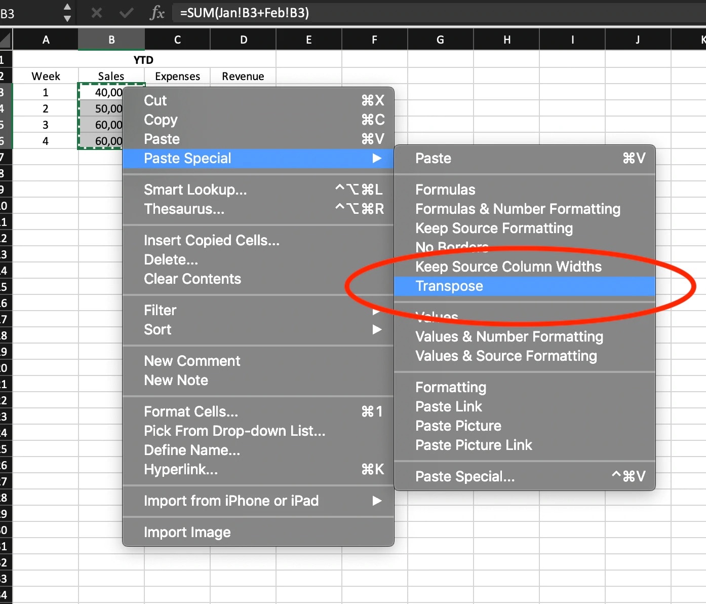
• Select the cell where you want to place the data, then right-click to get the dropdown menu. From that menu, select “Paste Special….”
• From the “Paste Special” menu, click the “Transpose” tickbox in the lower right-hand corner, then click “OK”. If you’re working on a Mac, it will look like the following screenshot.
• The data will flip with rows as columns and columns as rows

Excel trick no. 8: continue a series down a column or across a row

If you’re inputting a numbered list but don’t want to number every row, there’s a quick way to do it in Excel.

• Start your series of numbers.
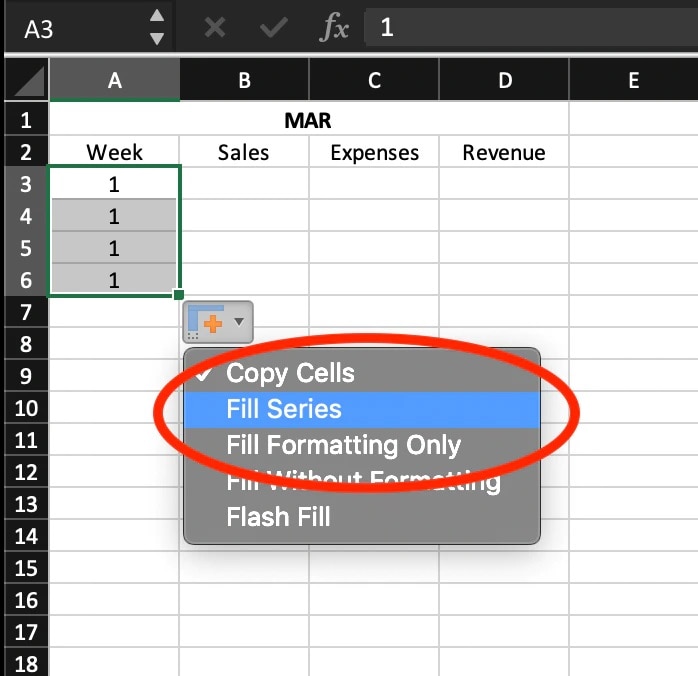
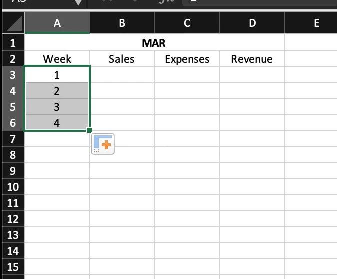
• Next, select the first cell in the list and drag down on the small box in the lower right-hand corner (similar to trick no. 6). The cells will auto-populate with what Excel believes you’re trying to do. (It can be intuitive and figure out that it’s a numbered list, a set of dates, etc.) But in the case below, you can see that it simply copied a “1” into each cell in the column, and that’s not what we want. So we’re going to need to make some changes.
• Right click, and a pop-up menu will show “Fill Series” as a second option. Click on that to change the settings.

This will adjust the values in the cells so that they become a numbered series. As shown below, the program will make this adjustment for however many cells you have highlighted. So, if you want it numbered from 1 to 100, highlight 100 cells.

Excel trick no. 9: highlight a list of numbers to see basic information

This Excel spreadsheet tip is a favourite of many Excel pros because it’s simple and so helpful, especially when dealing with figures and finances.

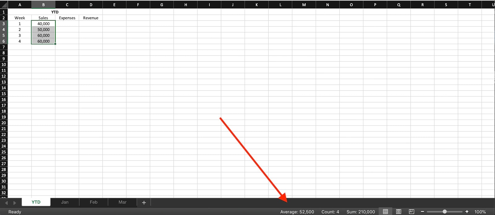
If you highlight a group of figures, Excel will display a few facts about them in the lower right-hand corner. There, you’ll see the number of highlighted cells, the total sum of the cells and the average of the cells’ values.

This Excel spreadsheet tip is really handy if you’re looking for a quick total or average without having to enter a formula.

Excel trick no. 10: essential shortcut keys and tips

One of the top Excel tips is getting acquainted with shortcuts. Here are some shortcuts that you may not be aware of. Some of these are universal across Microsoft Office products (e.g. Word, PowerPoint, etc.) but are still very helpful when using Excel.

• Ctrl + Z: this command undoes the last action you took in the worksheet. You can use the Ctrl + Z keyboard shortcut or the backwards arrow in the upper left-hand corner of the Excel window, above the navigation menu.
• Ctrl + Shift + up or down arrow: selects all of the cells directly above (up arrow) or below (down arrow) the selected cell. This only selects cells above and below that have data, so it won’t select empty cells.
• Shift + F11: creates a new worksheet in your current workbook called “Macro1”. This shortcut is also known as the insert tab shortcut. In Mac OS, you may need to add the Fn key for this shortcut to work.
• Ctrl + Home: navigates to cell A1.
• Ctrl + End: navigates to the last cell that contains data.
• Format Painter: select the cell whose format you want to copy. Then click on “Format Painter” (the little paintbrush) in the upper toolbar on the “Home” tab. Alternatively, you can click on the paintbrush in the pop-up format menu that appears when right clicking, then select the cell you want to format.
• Pivot table: a pivot table is a concise compilation of your input data, bundled in a visually understandable chart that can help you track and analyse data patterns. Pivot tables are ultra-useful tricks for Excel that effectively render a precise and multifaceted summary of thousands of rows and columns of unorganised data. By using pivot tables, you can organise vast volumes of information into an easily digestible spreadsheet. Use Excel keyboard shortcut Alt + N + V to quickly create a pivot table.

Making a new best friend in Excel

When starting a new business, you probably thought of the real dollar signs you’d work with, not the ones in your data tabs in Excel. But with these Excel tips and some perseverance, you’ll soon be filling those blank cells with data that allows you to quickly analyse your business’s progress. (As an added bonus, you’ll have a new sense of superiority around those new Excel users.)

Your journey towards using Excel and levelling up your management starts with that first column and will go on for years as you learn more advanced Excel functionalities. Now go forth, small business owner, and fill every single cell of your worksheets with reminders that your business exists and you are a rock star!

Hungry for more tips? Level up your spreadsheet skills by learning how to use Excel for accounting and bookkeeping. If you would like to see how QuickBooks could save you time, you can compare spreadsheet accounting to QuickBooks Online.