Tracking employee time in an Excel spreadsheet isn’t the easiest way to keep track of hours worked for payroll. For that, you might check out automated time tracking that integrates seamlessly with your payroll solution. But if you’re still shopping around and wondering if spreadsheets are right for you, download one of our free timesheet templates or learn how to create a timesheet in Excel. If you want to know how to create a timesheet template in excel, the following is a step-by-step guide to assist.
How to create a timesheet in Excel
A step-by-step guide to make a printable or digital timesheet
How to create an Excel timesheet
Every business has different needs. They depend on the type of work you do, how many people you employ, and about a hundred other variables. That’s why the first step to making a timesheet in Excel is to identify the categories you’ll need to create to run payroll—and your business—successfully. This timesheet includes space for employees to write down the following for each week.
- The date
- The job or shift
- The times they clock in (before and after lunch breaks)
- The times they clock out (before and after lunch)
- Their total number of hours
- The total number of overtime hours
- Their total number of sick hours
- Their total number of holiday hours
- Their total number of vacation hours
Your timesheet Excel might also include columns for answers to yes or no questions (e.g. Were you injured on the job? Is the project complete?) or space for client signatures.
Once you know which columns or labels you want in your timesheet, it’s time to create the working product. Here’s how to create a timesheet any employee can use.
Step 1: Format your spreadsheet
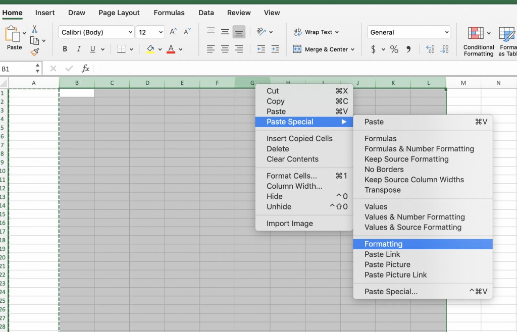
To create a spreadsheet that’s easy to read, first you need to format. Make all your cells wider, by first widening cell A (ours is set to 14.83). Then right-click on column A, select Copy, highlight columns B through L, right-click again, and select Paste Special, then Formatting.
Step 2: Title your timesheet
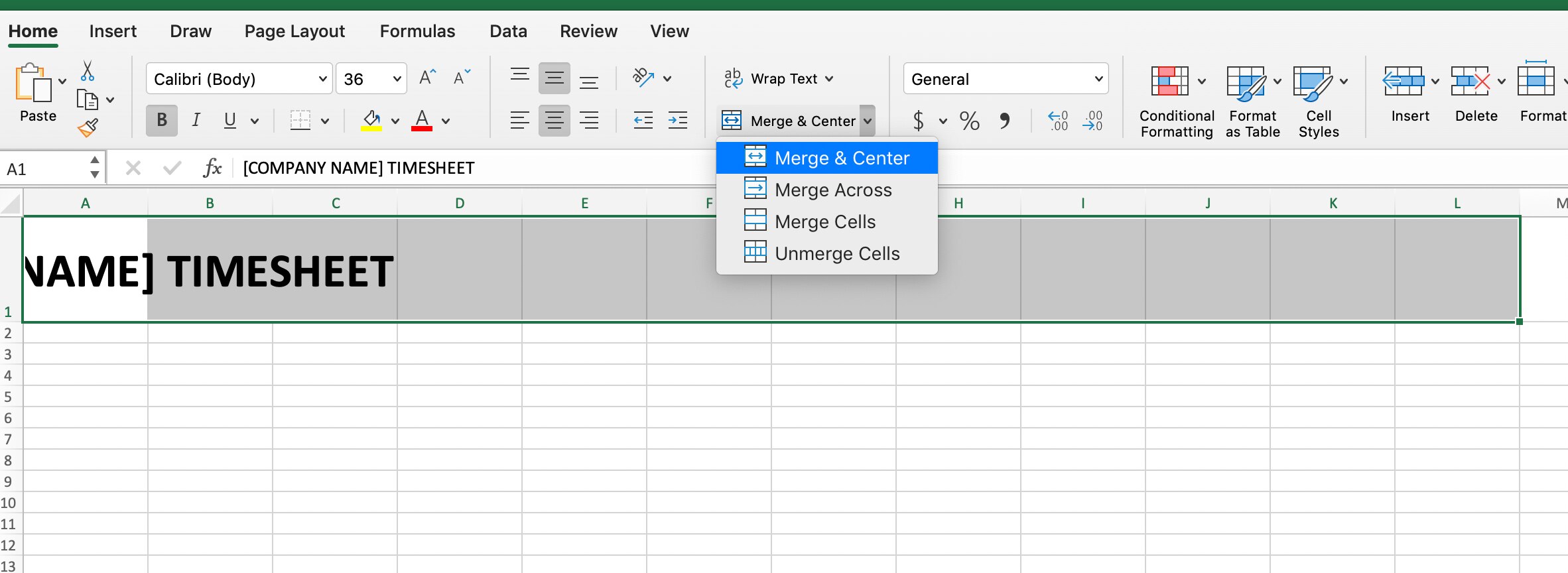
Type the name of your business into cell A1. Centre the text by width and height, and format the text by font, size (we used size 38), and colour, then bold it. Highlight cells A1 through L1. Select Merge & Centre on the Home toolbar.
Step 3: Add labels to your timesheet
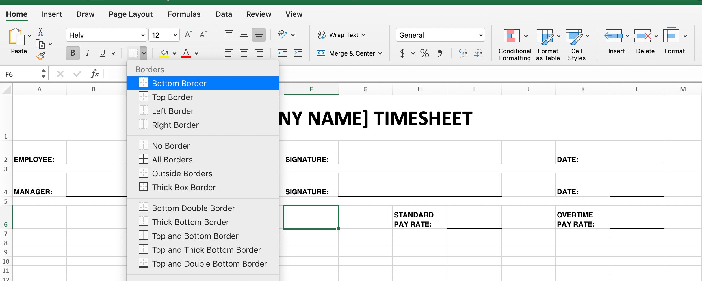
Add labels like EMPLOYEE and MANAGER (with signature and date lines for each), THIS WEEK’S START DATE, STANDARD PAY RATE, and OVERTIME PAY RATE. We used cells A2, A4, F2, F4, K2, K4, E6, H6, and K6.
For THIS WEEK’S START DATE, STANDARD PAY RATE, and OVERTIME PAY RATE, select Wrap Text, so the words don’t take up more than one cell.
In the cells following each label, make a line for employees and managers to write or type over by merging the cells and then applying a Bottom Border (from the borders tool, located on the Home toolbar). Merge cells A7 through L7 to create a small barrier between the next set of labels.
Step 4: Add timesheet labels
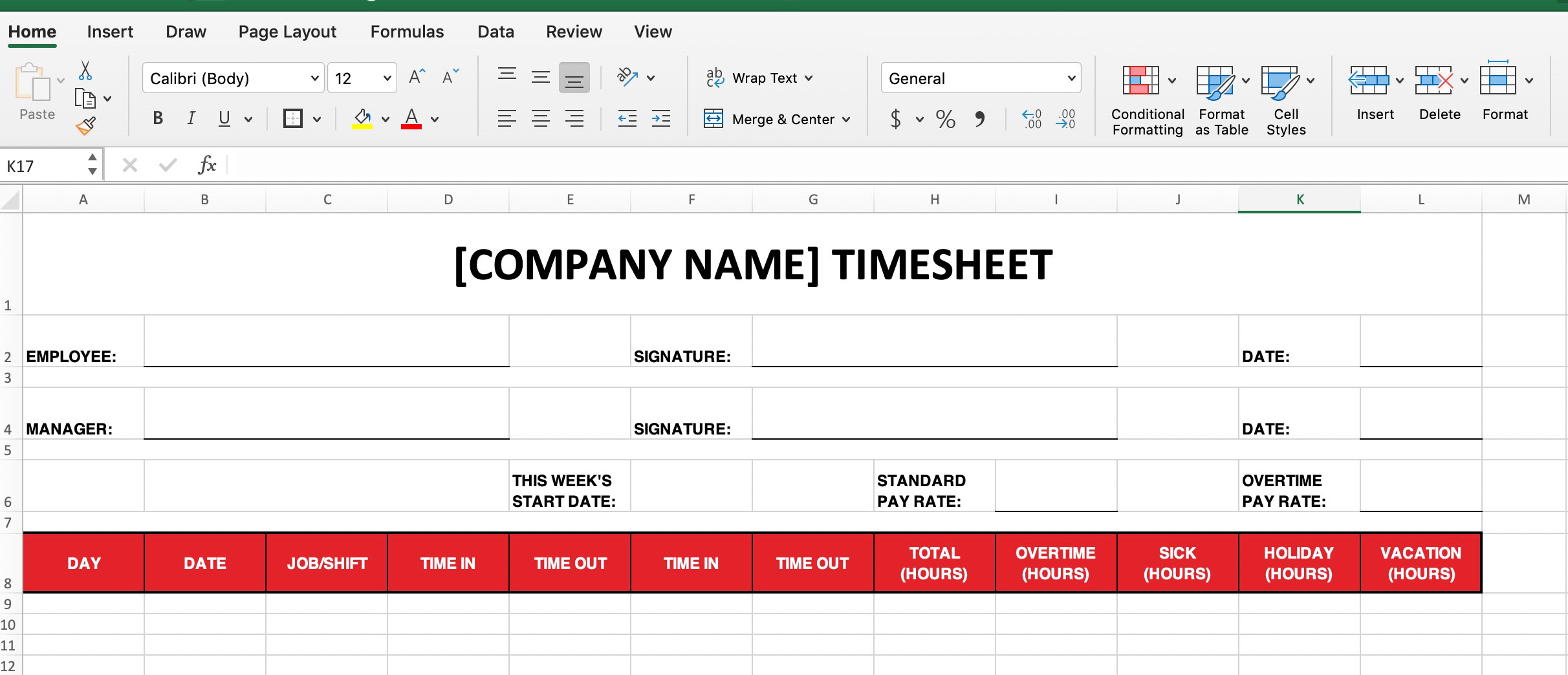
In row 8, create labels for each column: DAY, DATE, JOB/SHIFT, TIME IN, TIME OUT, TIME IN, TIME OUT, TOTAL (HOURS), OVERTIME (HOURS), SICK (HOURS), HOLIDAY (HOURS), and VACATION (HOURS). TIME IN and TIME OUT are listed twice to account for lunch breaks.
Fill the row with any colour of your choice, and use the borders tool to put boxes around the column labels. Center and bold the text.
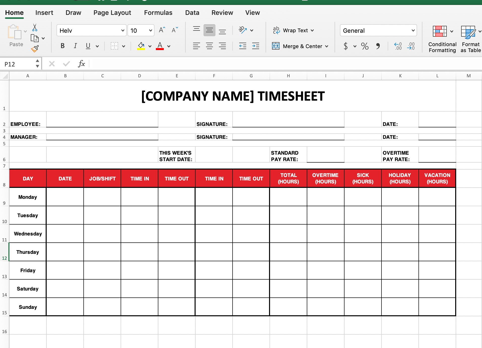
For this weekly timesheet, we’ve labelled the cells below DAY with the days of the week, starting with Monday in cell A9 and ending with Sunday in cell A15. Centre the labels up and down and side to side. Then widen rows 8 through 19 for better readability. Our rows are all about 46.00 high. Apply borders to all cells beneath the row of labels. Then add Thick Box Borders to better divide the table.
Step 5: Print the timesheet
If your plan is to print this template and have employees turn in handwritten timesheet data, you’re almost done!
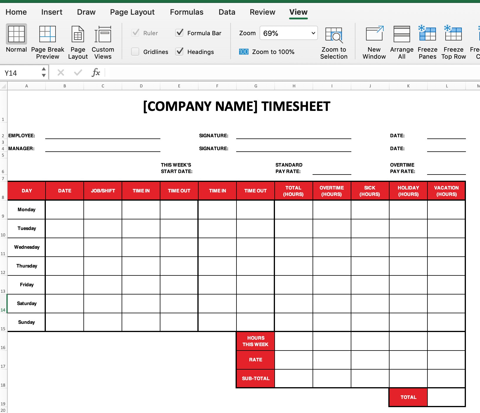
The last thing you need to do is set up labels for totals. In cells G16, G17, and G18, write HOURS THIS WEEK, RATE, and SUB-TOTAL. In cell K19, write TOTAL. Make these cells whatever colour you like, then centre and bold the text. Use the borders tool to make these sections stand out.
Put some final spit and polish on your document by removing any unnecessary gridlines. Select View and uncheck the box that says Gridlines.
Now you can print copies of this Excel timesheet for employee use.
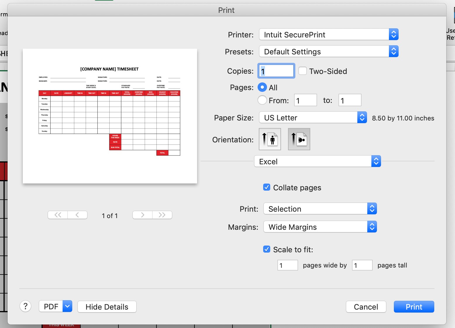
- Highlight everything you want printed (A1 across to L1 and down to row 19).
- Click on File > Print > Show Details
- Select landscape orientation
- Under Print, choose Selection
- Under Margins, choose Wide Margins
- Check the box that says Scale to fit and click Print
That’s it—you’re done! Don’t want to print? Keep reading.
How to add formulas for automatic calculations
This is where we start making spreadsheet magic. Assuming you haven’t removed or added any days to your spreadsheet, HOURS THIS WEEK should be in cell G16, while TOTAL should be in cell K19.
Step 1: Prepare to add formulas for digital use
Follow instructions from step 5, then highlight cells H16 over L16 and down to row 18. Turn these and cell L19 grey. Now the boxes with your calculations will stand out from the rest of the employee’s timesheet entrees.
Step 2: Click on cell H16 or whatever cell is directly beside the box that says HOURS THIS WEEK. In the formula bar, type in =SUM(H9:H15) and press Enter. This box will now add any numbers entered in the column labelled TOTAL (HOURS).
Step 3: Click on cell I16. In the formula bar, type in =SUM(I9:I15) and press Enter. This box will now add any numbers entered in the column labelled OVERTIME (HOURS).
Step 4: Click on cell J16. In the formula bar, type in =SUM(J9:J15) and press Enter. This box will now add any numbers entered in the column labelled SICK (HOURS).
Step 5: Click on cell K16. In the formula bar, type in =SUM(K9:K15) and press Enter. This box will now add any numbers entered in the column labelled HOLIDAY (HOURS).
Step 6: Click on cell L16. In the formula bar, type in =SUM(L9:L15) and press Enter. This box will now add any numbers entered in the column labelled VACATION (HOURS).
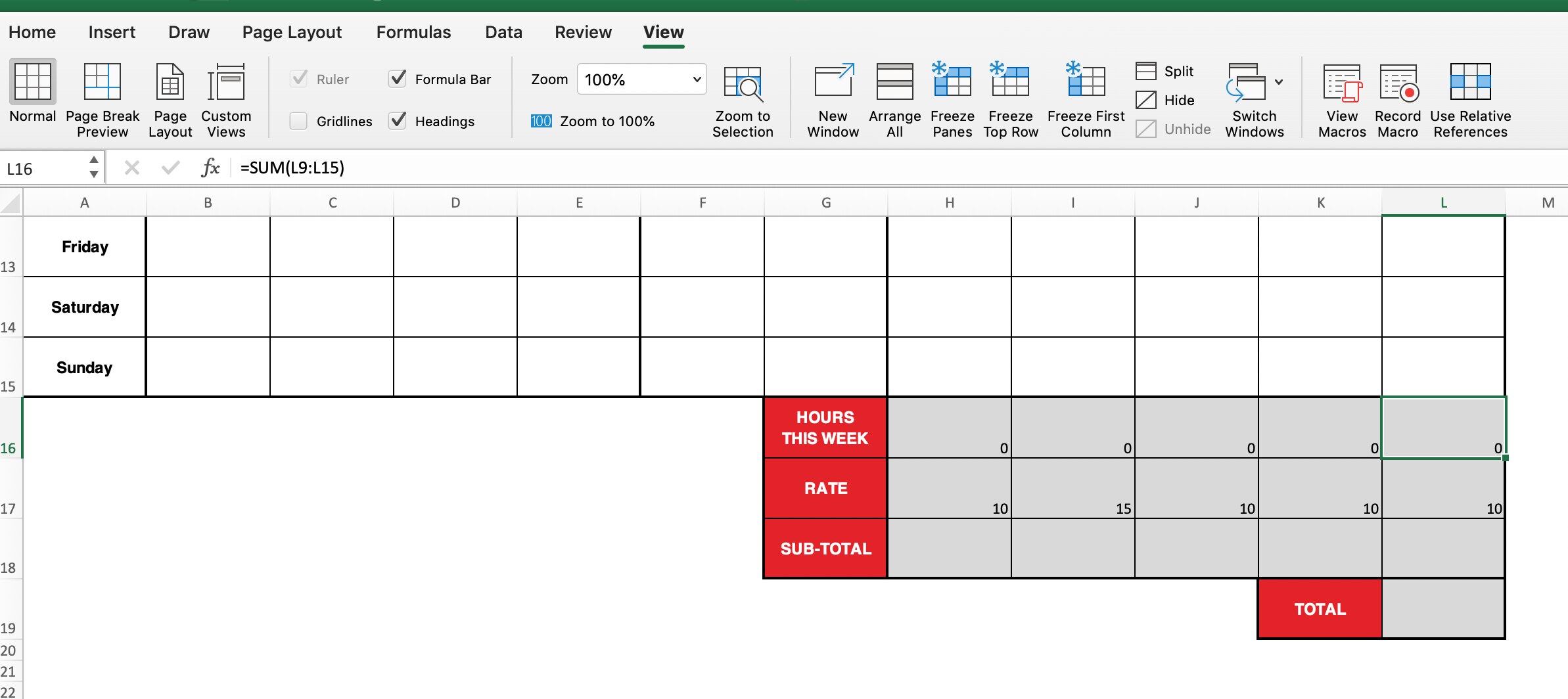
Step 7: In cell H17 (or whatever cell is directly beside RATE), type in the employee’s hourly rate. In the cell beside that, type in the employee’s overtime rate.
If your business provides paid time off (PTO) for sick time, vacations, and holidays, fill J17, K17, and L17 with the employee’s standard hourly rate.
As an example, if your employee makes $10 per hour, the bottom of your spreadsheet will look like this:
Step 8: Now to calculate sub-totals. Click on cell H18 (or whatever cell is directly beside SUB-TOTAL). In the formula bar, type in =SUM(H16*H17) and press Enter. This box will now multiply the employees total hours by their standard pay rate to show how much money they’re owed.*
Step 9: Click on cell I18. In the formula bar, type in =SUM(I16*I17) and press Enter. This box will now multiply the employee’s overtime hours by their overtime pay rate to show how much they’re owed.*
Step 10: Click on cell J18. In the formula bar, type in =SUM(J16*J17) and press Enter. This box will now multiply the employee’s paid sick hours by their standard pay rate to show how much money they’re owed.*
Step 11: Click on cell K18. In the formula bar, type in =SUM(K16*K17) and press Enter. This box will now multiply the employee’s paid holiday hours by their standard pay rate to show how much money they’re owed.*
Step 12: Click on cell L18. In the formula bar, type in =SUM(L16*L17) and press Enter. This box will multiply the employee’s paid vacation hours by their standard pay rate to show how much money they’re owed.*
For example, say an employee worked 42 hours this week. Cell H16 should now say 40, while cell I16 should say 2. If your formulas are correct. H18 will say 400, while I18 will say 30.
*These are basic calculations and do not include things like taxes, workman’s comp, or other paycheck deductions.
Step 13: At last, we get to calculate the total money owed. Select cell L19. In the formula bar, type in =SUM(H18:L18) and press Enter. This box will now add the five sub-totals to show how much money your employee has made total (before bonuses,
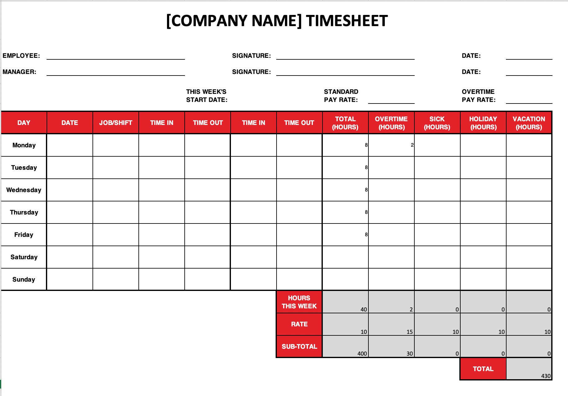
Now you know how to make a timesheet in excel. Think that’s simple? Check out our digital timesheet solution with easy integrations to QuickBooks, ADP, and other payroll providers. And keep in mind, paper timesheets are the leading cause of timesheet errors. An automated time tracking tool like QuickBooks Time could save your business time and money every time you run payroll—and grant you more peace of mind.
Need a more sophisticated solution, QuickBooks Time can help
Time tracking for your small business can be made easier with QuickBooks Time. QuickBooks Time can help your small business track time, manage teams and projects and help reduce the time it takes to run payroll.
- Employees can clock in and clock out through their mobile (via QuickBooks Workforce, the QuickBooks Time Mobile app) or a fixed location tablet at your shop or building site (via the Time Clock Kiosk)
- Managers can create & share rosters with teams in minutes
- GPS time tracking can be used to keep track of remote teams.
Get a free 30-day trial to QuickBooks time now.
