41 best Excel tips and tricks to save you time

From meticulously tracking expenses to crunching sales figures, Microsoft Excel is the unsung hero of many small business toolkits. For some, it’s a powerful ally, turning raw numbers into clear insights. For others, it's more of an untamed jungle of unstructured data and confusing file types, that has business owners shaking in their boots. 

If that describes you, we have good news. We've compiled a list of our favorite smart and handy Excel tips and tricks to save you time scouring the internet for spreadsheet tips.

These Excel tips are great for speed, but comparing excel vs accounting software shows that while Excel can be tuned with shortcuts, the fundamental limitations remain: accounting software handles repetitive tasks, version control, and financial compliance more robustly. So use these tricks to boost your spreadsheet work, but keep in mind that for full financial accuracy and scale, accounting software may be the safer long-term choice.

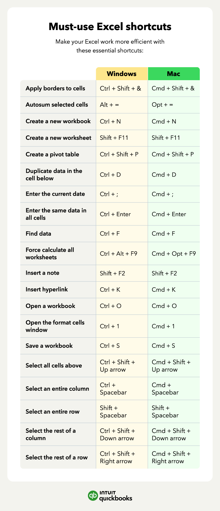
If you're ready to become an Excel wizard, or at least wrap up that timesheet template you've been working on forever, read on to unlock some of the fastest Excel shortcuts on the internet. 

Jump to:

• Excel basics: 7 Formulas and functions
• Excel keyboard shortcuts
• Data selection and formatting Excel tricks
• How to use Excel for efficiency
• Excel how-to for data analysis and visualization
• Excel data protection and integration
• Spend more time growing your business

Excel basics: 7 Formulas and functions

When first learning how to use an Excel spreadsheet, it’s best to start with simpler formulas and functions that can improve your productivity:

1. Use formulas for simple calculations

Excel's built-in formulas make it easy to perform all sorts of calculations, from basic arithmetic to complex functions. Whether you need to calculate employee hours or an average price, Excel's formulas can save you time and ensure accurate results.

For example, if you want to sum the numbers in a range from E2 to E9, you can type "=SUM(E2:E9)" in a cell and press Enter. The sum of the numbers will appear in the cell.

2. Try the IF formula to automate Excel functions

The IF formula is a powerful tool for automating certain Excel functions. With this formula, you can specify different values or actions depending on whether a particular condition is true or false. 

The formula is =IF(logical_test, value_if_true, value_if_false), where: 

• The logical test is the condition that you want to evaluate.
• The value_if_true is the result or action to be taken if the condition is met or true. 
• The value_if_false is the result or action to be taken if the condition is not met or false. 

For example, you can check if a cell value is greater than a certain number.

3. Test VLOOKUP to pull data across sheets

The VLOOKUP function helps you extract data from one part of your spreadsheet and display it elsewhere. This is especially useful when you have data spread across multiple sheets.

For example, say you enter the VLOOKUP formula: "=VLOOKUP(A2, Sheet2!A:B, 2, FALSE)" into your sheet. The formula will search for the value in cell A2 of your current sheet in Sheet2 and return the corresponding value from the second column.

4. Use INDEX and MATCH formulas for horizontal data

When working with data arranged horizontally, the combination of the INDEX and MATCH functions can be more efficient than VLOOKUP. This approach allows you to look up values based on both row and column criteria, making it a powerful tool for complex data analysis. In this case, you’ll use the INDEX formula and include the MATCH formula within it.

5. Have COUNTIF count words or numbers

The COUNTIF function, which is =COUNTIF(range, criteria), is a great way to count the occurrences of specific words, numbers, or other criteria within a range of cells. This can be helpful for tasks like inventory management and identifying trends.

6. Combine cells with the (&) operator

The ampersand symbol, &, allows you to combine the contents of multiple cells into a single cell. This can be useful for tasks like merging first and last names, creating full addresses, or assembling various data points.

7. Use named ranges for easier formulas

Assigning meaningful names to cell ranges or cells can make your formulas more intuitive and easier to understand. Named ranges also let you reference cells by their descriptive names rather than cell addresses, simplifying formula-building. 

To use named ranges, start by selecting the cells you want to name, navigate to the Formulas tab, and select Define Name. 

Excel keyboard shortcuts

Excel is full of shortcuts that can help make navigating your sheets easier—especially when you're using Excel for accounting.

8. Create a new workbook

To quickly create a new Excel workbook, use the keyboard shortcut Ctrl + N for Windows or Cmd + N for Mac. This will open a new, blank Excel workbook ready for you.

Note that this is different from a worksheet. To create a new worksheet within your current workbook, you can use Shift + F11 on Windows and Mac.

9. Select an entire row

To select an entire row, simply press the Shift + Spacebar on your keyboard. This will highlight the entire row and the selected row will typically turn a different color to indicate its selection, such as a light blue. Selecting an entire row allows you to apply formatting, copy and paste, or delete rows quickly, without making individual cell selections.

10. Select an entire column

To select an entire column, press Ctrl + Spacebar on Windows or Cmd + Spacebar on Mac. Like the select an entire row shortcut, it allows you to quickly make a selection to manipulate, format, or analyze data.

11. Select the rest of a column

If you need to simply select the rest of a column versus the entire column, click on the cell you’d like to start and press Ctrl + Shift + Down Arrow on Windows or Cmd + Shift + Down Arrow on Mac.

12. Select the rest of a row

Selecting the rest of a row versus an entire row can be done by clicking on the cell you want to be the starting point, then pressing Ctrl + Shift + Right Arrow on Windows or Cmd + Shift + Right Arrow on Mac.

13. Add a hyperlink

To quickly add a hyperlink to a cell in Excel, press Ctrl + K in Excel for Windows or Cmd + K for Mac. Adding a hyperlink is useful for quick access to external files, websites, or specific locations within the same

14. Open the format cells window

To open the Format Cells window, press Ctrl + 1 on Windows or Cmd + 1 on Mac. This window will allow you to modify cell formatting, including changes to fonts, borders, and number formats.

15. Autosum selected cells

To quickly sum up a range of selected cells in Excel, press Alt + = for Windows or Opt + = for Mac. Autosum is a handy feature in Excel that allows you to quickly calculate the sum of selected cells. This is useful when working with large data sets or analyzing financial information.

Data selection and formatting Excel tricks

When adding data to your Excel spreadsheet, you can quickly format and update your cells with a few shortcuts:

16. Add multiple rows or columns

To insert multiple rows or columns, select the number of rows or columns you want to add, right-click, and choose "Insert.”

Excel will automatically add the same number of rows or columns that were highlighted and shift the existing data down or to the right to accommodate the new additions. This method is especially useful when a large number of rows or columns need to be added.

17. Use filters to simplify data

Applying filters to your data allows you to quickly sort, search, and analyze information—making it easier to find and work with the data you need. To add a filter in Excel, simply click on the Data tab in the toolbar and select "Filter.” This will add drop-down Arrows next to each of the column headers in your data. 

For example, if you have a spreadsheet with a column for sales data and you want to see only the sales figures that are above a certain threshold, you can add a filter to that column and select the criteria for displaying only the rows that meet that threshold.

18. Transpose rows to columns

To convert a range of rows into columns (or vice versa), select the row or column you want to transpose, right-click on the column header, and choose the "Copy" option. Next, select the cell where you want to start transposing the data, right-click, choose “Paste Special,” and select “Transpose.”

19. Split text into separate columns

You can split text data in a single cell into multiple columns by using spaces or commas. Select the column, go to the “Data” tab, and click "Text to Columns.” You can choose the delimiter, such as a comma, that separates the text you want to split. For example, select the "Comma" option if the text is separated by commas.

20. Use conditional formatting for color coding

Conditional formatting enables you to automatically apply different colors, icons, or data bars to cells based on their values or criteria you define. This can help you quickly identify patterns, trends, and outliers in your data.

In the "Home" tab of the Excel ribbon, click the "Conditional Formatting" button. Excel offers a wide range of options, such as highlighting cells that contain specific text or are greater than or less than a certain value.

21. Add checkboxes

You can add checkboxes to your spreadsheet to allow users to indicate the status or selection of specific items. Having checkboxes can be useful for tracking tasks or selection options. 

Note: You need the “Developer” tab to do this. If you don't see the "Developer" tab, you may need to enable it first. To do this, you need to click “Excel” and go to "Preferences," then select “Ribbon & Toolbar” and find “Developer” under the “Customize the Ribbon” column. 

Now go to the “Developer” tab, click “Insert,” and select the checkbox option.

22. Try the format painter

The format painter tool allows you to quickly copy formatting from one cell or range to another, saving you time on repetitive formatting tasks. Simply select a cell and format it as you’d like. Select the cell or range of cells with the formatting you want to copy and click the "Format” button in the Excel toolbar. Then, select the cell or range of cells where you want to apply the formatting. 

23. Group data for better organization

Grouping related rows or columns can help you expand and collapse sections of your spreadsheet, making it easier to navigate and analyze complex data. Select the range of cells or columns you want to group and go to the “Data” tab in the Excel ribbon. 

Look for the “Group” button, and after clicking it, you can specify the grouping levels you want. For example, if you have a dataset with dates, you can group it by months, quarters, or years.

24. Use Find & Select to streamline formatting

The "Find & Select" feature provides advanced options for locating and formatting specific cells or data types within your spreadsheet. This allows you to quickly locate specific data in your spreadsheet and make formatting changes with ease.

 To use the “Find & Select” tool, first, navigate to the “Home” tab in the Excel ribbon, then select the “Find & Select” drop-down menu.

25. Create custom number formats

Excel's built-in number formats can be customized to display data in various ways, such as currency, percentages, or custom date and time formats. To create custom number formats in Excel: 

• Select the desired cell or range where you want to apply the custom number format.
• Right-click and choose the "Number Format" option from the context menu. 
• Click on the "Custom" category and enter your customer number format. 

For example, if you want to display the number with two decimal places, you can enter the format code 0.00.

26. Improve presentation with text wrapping

Wrap text within a cell to ensure that long entries are fully visible and your spreadsheet maintains a clean, organized appearance.

Text wrapping is particularly useful when working with lengthy sentences or paragraphs within cells. It allows you to display the full content of the text while maintaining the cell's width. On the "Home" tab of the toolbar, select the “Wrap Text” button.

27. Add emojis

You can liven up your spreadsheets by inserting emojis into cell contents, headers, or comments to add a touch of personality and emphasis. Depending on your operating system, you can open the emoji keyboard using the keyboard shortcut. For Windows, use Win + . or Win + ; and for Mac use Ctrl + Cmd + Space.

How to use Excel for efficiency

You can use Excel tricks to efficiently analyze data to get quick insights about your business:

28. Use pivot tables to analyze data

Pivot tables make inventory management in Excel a snap. They are powerful tools for analyzing and visualizing large datasets. They allow you to quickly reorganize and aggregate your data, such as product sales or inventory, to uncover insights and trends.

To create a pivot table, start by selecting the data range you want to analyze. Then, from the "Insert" tab on the Excel ribbon, click on the "PivotTable" option. 

Once the pivot table is created, you can manipulate the data further by applying various functions like sum, average, or count to the values. You can also sort, filter, or format the data to present it in a more meaningful way.

29. Customize the Excel ribbon

You can personalize the Excel ribbon by adding your most-used commands and tools to the quick-access toolbar or by creating custom ribbon tabs and groups. This can streamline your workflow and improve efficiency.

To customize the Excel ribbon, go to “Excel” and select “Preferences.” From there click “Ribbon & Toolbar” and from there you can add, remove, and rearrange tabs and commands to the ribbon. 

30. Freeze panes to keep headers visible

When working with large spreadsheets, you can freeze the top row or leftmost column to ensure that your column and row headers remain visible as you scroll through the data. Navigate to the View tab on Excel and look for the freeze options, such as “Freeze Panes.” 

For example, to keep the headers visible, choose either the "Freeze Top Row" or "Freeze First Column" option, depending on your preference.

31. Use Flash Fill for quick data fills

The Flash Fill feature in Excel can automatically populate cells based on a pattern you establish, saving you time on repetitive data entry tasks. To flash fill, ensure that you have data in a column or columns with a discernible pattern. 

Go to the "Data" tab and click the "Flash Fill" button. Alternatively, you can use the keyboard shortcut Ctrl + E for Windows or Mac.

32. Split data with text to columns

Similar to the "Split Text into Separate Columns" tip, converting text to columns allows you to separate concatenated data into individual columns quickly. Highlight the column that contains the data you want to split. Then, navigate to the "Data" tab in the Excel ribbon and click on the "Text to Columns" button. 

Choose the appropriate option depending on the structure of your data. For example, if your data is separated by a specific delimiter, such as a comma, tab, semicolon, or space, select "Delimited.”

Excel how-to for data analysis and visualization

Figuring out what Excel is used for also means learning to utilize the program for data analysis and visualization. It's essential territory for any Excel guide. 

33. Customize your data tables

Excel's data table features enable you to quickly adjust the appearance and functionality of your tables, such as adding total rows, filtering options, and custom styles. You can quickly do this by going to the “Home” tab in the Excel ribbon and selecting “Format as Table.” Excel will automatically apply the selected style to your selected range of cells.

34. Add drop-down menus

Creating a dropdown list in your spreadsheet helps ensure data consistency and prevent user input errors. Select the cells where you want the drop-down menus to be, go to the “Data” tab, and click “Data Validation.”

In the settings box, you'll see various options. Here, you choose the lists option and enter the values that you want to appear in the drop-down menu.

35. Save chart templates

You can also create custom chart templates to quickly generate visually consistent and professional-looking visualizations in your spreadsheets. For example, to save chart templates in Excel, follow these steps:

• Create and perfect the desired chart in Excel
• Right-click on the chart and select "Save as Template" 
• Navigate to the default Microsoft Excel Templates folder
• Name your template and save it 

When creating a new chart you can find your saved template in the “Templates” folder.

36. Use graphics in charts

You can enhance your charts and graphs by incorporating relevant icons, images, or other visual elements to make your data more engaging and impactful. Simply select your chart, go to the “Insert” tab, and click “Pictures” to insert a picture. Note you can also place graphics on bars and pie slices and use clip art.

37. Create sparkline mini-charts

Sparklines are small, inline charts that can be used to visualize trends and patterns within your data, providing a compact and informative way to display metrics. 

To create sparkline mini-charts use the “Insert” tab in the Excel ribbon and click "Sparklines," then the type of sparkline you want to create. You can then customize the appearance of the sparkline mini-chart.

Excel data protection and integration

When creating Excel sheets, one trick to keep your data safe is with protections:

38. Protect a worksheet

You can secure your data by password-protecting individual worksheets, preventing unauthorized access or accidental changes. To protect a worksheet, go to the “Review” tab and select "Protect Sheet.” Here you can create a password or set permissions for users to do specific actions like sort and filter data.

39. Protect a workbook

In addition to protecting individual sheets, you can also password-protect an entire Excel workbook. To protect a workbook, go to the “Review” tab and click "Protect Workbook." You can prevent users from adding, deleting, hiding, or renaming worksheets, as well as moving or copying worksheets to another workbook.

40. Insert Excel data into Word

Easily embed your Excel data, charts, and tables directly into Microsoft Word documents, allowing you to combine your spreadsheet analysis with written reports or presentations. You can do this easily by copying the data in Excel and simply pasting it into your Word document. 

Note that you can also paste the data as a picture in Word using the “Paste Special” feature and choosing to paste it as a picture.

41. Try AI Copilot in Excel

You can leverage the power of artificial intelligence with Excel's Copilot feature, which can assist you with various tasks like formula generation, data analysis, and even creative ideation. AI Copilot is an innovative tool that integrates artificial intelligence capabilities into Excel. You can also use artificial intelligence in accounting with tools like Intuit Assist.

Spend more time growing your business

When you first dreamed of starting your business, you probably envisioned big ideas, serving customers, and seeing those real dollar signs grow, not the virtual ones in Excel data tabs. 

But here's the good news: with this Excel tips and tricks cheat sheet, you'll soon fill those blank cells with meaningful data that empowers you to analyze your business's progress. And the journey doesn't have to stop there—you can also learn to use Excel for bookkeeping.

If you still haven't taken to Excel, you can skip the data entry entirely and use accounting software like QuickBooks Online to streamline your finances. QuickBooks is automated and helps you run your business more efficiently and error-free.